Flow Through Pipes, Fittings, and Pressure Measurement Devices
Introduction
This discussion will be split into 3 parts, mirroring the format of the lab manual document provided to you. The first part of this discussion will look at the flow through tubes and pipes. Here will look at the relationship between the Darcy friction factor and the Reynold’s number. Here we will begin to develop our understanding of the effect the roughness of a pipe has on the head loss in the system.
The second part of this discussion, we will be investigating the volumetric flow rate through a venturi meter and orifice plates, devices used to measure the flow rate of a fluid. Specifically, we will be examining the pressure drop across these flow meters to examine any head loss and how these devices can measure the flow rate in the system.
The last part of this discussion will be looking at energy losses (head losses) surrounding fittings like bends, globe valves, contractions and expansions, etc. We will be looking at how to examine the extent of energy loss each fitting can incur on the system, and look at ways on how to design against these energy losses efficiently.
Flow Through Pipes
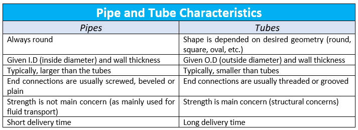
We start our discussion by first distinguishing the difference between pipes and tubes. This is so that we can narrow the scope of our discussion to specific systems that you will be examining during your labs. The different characteristics of both a pipe and tube are summarized below:
Fluids can be described as either ideal or real. Ideal fluids are characterized by having zero internal forces (essentially zero viscosity), which don’t actually exist. We can regard fluids to be ideal in system if the internal friction forces are negligible to the external frictional forces.
We know that there are 3 regions for flow regimes, where each regime is separated by the Reynold’s number. The laminar flow regime occurs when the Reynold’s number is below 2000 (Re < 2100). Here, streamlines do not cross and no vortices are created (shown below).
As we can see from the image, the streamlines are ordered and seem to be organized. This indicates a simple velocity profile as the fluid particles are not oriented randomly in this flow regime. We can model the velocity profile for this flow region as the following:
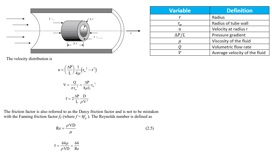
In the laminar region, we can attribute most of the friction due to internal forces, i.e. we can attribute most of the friction to the viscous effects of the fluid. Since the viscous effects dominate the friction the fluid experiences, we can see that the roughness of the pipe does not affect the pressure drop the fluid experiences.
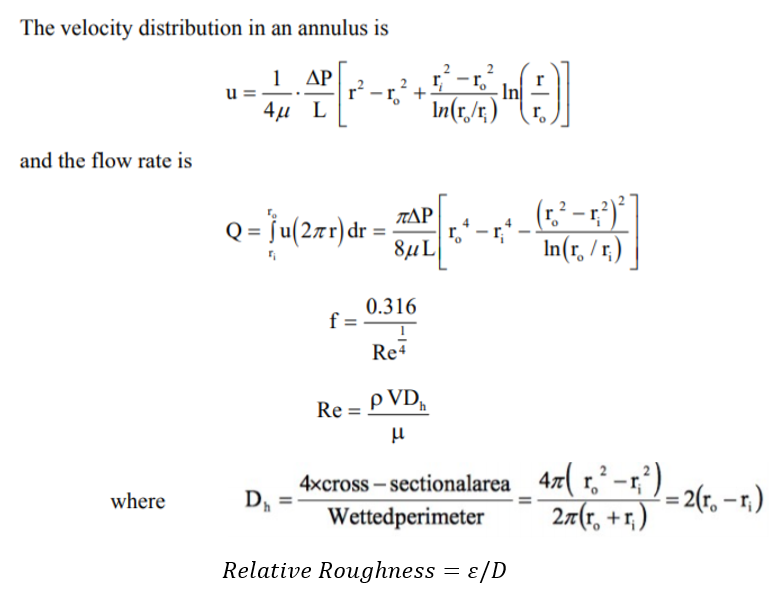
Hence, we must examine the turbulent region to see the effects of the roughness of the pipe on pressure drop. The flowing fluid is said to be in the turbulent region when the Reynold’s number is bigger than 4000 (Re > 4000). In this region, the viscous effects do not dominate the friction a fluid experiences. The viscous effects are generally only present at a laminar sublayer closer to the edge of the pipe. The roughness of the pipe can intrude on to this laminar sublayer. What actually occurs is that the laminar sublayer begins to become smaller and smaller with an increasing Reynold’s number. The smaller the sublayer, the more the roughness of the pipe will affect the shear stresses the fluid will experience (and therefore its pressure drop too).
The first equation, which determines the Darcy factor, is only valid for completely smooth pipes. For any pipe with a certain amount of roughness, we must include a correction factor to determine the real friction factor. Here, we calculate the Reynold’s number and the relative roughness of the system. We then use these two values to determine the real friction factor.
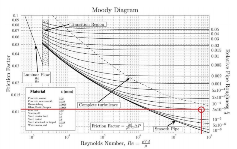
Each already drawn line on the graph represents a certain relative roughness. Following the calculation of relative roughness, determine which line represents this relative roughness value. Draw a vertical line up from the Reynold’s number value that corresponds to the system we our examining. This line is represented by the vertical red line. If we then draw a horizontal red line from this point of intersection, we can find the corresponding friction factor to the system.
We can then calculate the head losses (pressure drop equivalent in height of working fluid) using the following equation:
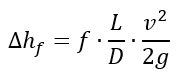

Knowing this head loss, we gain a better understanding of energy losses and pressure drops in our system. Knowing this piece of information brings us one step closer to design a pump that overcome the head losses in the system so that the flow of material in the system remains efficient.
Flow Through a Venturi Meter and an Orifice Plate
These devices are commonly found in any plant with a flow system. We use these measurement devices to measure the flow rate in a pipe. They do this by generating a large, local (exist for a short amount of time) changes in pressure. Using the pressure difference, the device is able to correlate the pressure drop to the velocity of the flow.
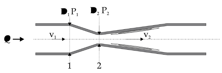
Venturi meter, where points 1 and 2 indicate where we measure the pressure drop
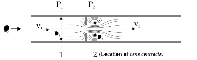
Venturi meter, where points 1 and 2 indicate where we measure the pressure drop, and location 2 is where the vena contracta is present.
The figures above show the different configurations each device has. The venturi meter consists of a constricted region (from points 1 and 2) and a divergent section (point 2 and onward). The constriction forces the fluid to move faster (through principle of conservation of mass) and cause for a corresponding pressure drop. Using this pressure drop (P1 – P2), we can calculate the initial inlet velocity to the venturi meter.
The orifice plate works by a similar principle. Here when the fluid reaches the small hole in the plate, fluid builds up to the left of the plate, causing for the pressure to build up. The velocity of the fluid flowing through the hole begins to increase, so the pressure on the right begins to decrease. Again, we see the same concept being applied. The meter uses the pressure difference (P1 – P2) and corresponds it to a specific fluid flow. The vena contracta here is describing the location where the streamlines have their smallest diameter and fastest velocity (which is right after the fluid flows past the orfice plate).
It has been found that in an orifice plate and venturi meter, is is difficult to theoretically predict the friction factor for this system. Instead, engineers use a coefficient of discharge value that not only encapsulates the energy loss due to friction, but also relates the flow in and out of the device.
Before looking at this effect, let’s examine the system with the absence of friction. From CHE211, we know that for a horizontal system (our devices), the bernoulli equation states:
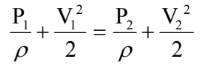
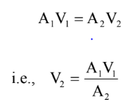
The Bernoulli equation assumes that it is inviscid flow (ideal, incompressible fluids) present in the system. The continuity equation can the be simplified as shown above.
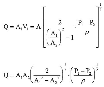
Substituting the the outlet velocity equation into the Bernoulli equation, we define the inlet velocity and flow rate to the devices with the following equations:

Since we have developed all these equations from the continuity and bernoulli equations, the fluid is still assumed to be ideal and incompressible. However, it is worth noting that the venturi meter constricts the fluid as it enters the device, but downstream (after the fluid has exited the device) the fluid expands, which is a non-ideal property. The system isn’t entirely ideal. The same can be said for an orifice plate, but for a different reason. Remember the vena contracta? The fast velocities there, including the low diameter of streamlines, there is considerable turbulent motion surrounding it, which leads to friction losses.
To account for this non-ideality, we include what we have discussed before: a coefficient of discharge. The equation form of this principle is shown here:

To determine the value of this coefficient, we can experimentally determine the relationship between the flow rate, Q, and the pressure drop, (P1 – P2). Using spreadsheet software (like Microsoft Excel), you can plot the data on a logarithmic scale for flow rate on the y-axis and pressure drop on the x-axis. The results will show a linear relationship with a slope of 1/2 and an intercept of Cd. I’ve actually simplified this since if you actually looked at the math, you can see it gets quite messy. But we still want the relationship between pressure drop and flow rate so we can design our system. Instead, we can set the intercept to simply the overall constant discharge coefficient between flow rate and pressure drop. The equation would simply be:

Flow Through Pipe Fittings
Pressure drops and energy losses through pipe fittings are known as minor losses. Major losses exist and is defined as the energy lost to friction from the pipe itself. Major losses can be found experimentally by just running the whole system and measuring various parameters to find the friction factor for the whole system. Minor losses encapsulates energy losses of flow through pipe fittings like globe valves, bends, etc.
The pressure drop across a fitting is expressed as follows:

At high flow rates, flow though a pipe fitting is independent of viscous forces. The flow mainly driven by inertia. Under these conditions, the friction factor becomes independent of the Reynold’s number, which is why you don’t see the friction being a function of Re. Tables can be found showing what has been experimentally found for each loss coefficient of each fitting at different orientations.